Code
library(tidyverse)
library(gt)
library(rstan)

options(mc.cores = parallel::detectCores())
rstan::rstan_options(auto_write = TRUE)library(tidyverse)
library(gt)
library(rstan)
options(mc.cores = parallel::detectCores())
rstan::rstan_options(auto_write = TRUE)ns_full <- rio::import("https://raw.githubusercontent.com/forecastingresearch/fpt/refs/heads/main/data_cognitive_tasks/task_datasets/data_number_series.csv")
session <- rio::import("https://raw.githubusercontent.com/forecastingresearch/fpt/refs/heads/main/data_cognitive_tasks/metadata_tables/session.csv")ns_dat <- ns_full |>
left_join(session,
by = "session_id") |>
left_join(rio::import("https://raw.githubusercontent.com/forecastingresearch/fpt/refs/heads/main/data_forecasting/processed_data/scores_quantile.csv") |>
select(subject_id, sscore_standardized) |>
# mean sscores per person
summarize(.by = subject_id,
sscore = mean(sscore_standardized)),
by = "subject_id") |>
mutate(ns_id = tolower(ns_id),
# if no response, incorrect
correct = ifelse(is.na(correct), 0, 1)) |>
select(subject_id, ns_id, score = correct, sscore)
if (!file.exists(here::here("Data", "Number Series"))) dir.create(here::here("Data", "Number Series"))
saveRDS(ns_dat, here::here("Data", "Number Series", "ns_dat.rds"))ns_labels <- tribble(~item_label, ~series,
"NS_1", "10, 4, _, -8, -14, -20",
"NS_2", "3, 6, 10, 15, 21, _",
"NS_3", "121, 100, 81, _, 49",
"NS_4", "3, 10, 16, 23, _, 36",
"NS_5", "3/21, _, 13/11, 18/6, 23/1, 28/-4",
"NS_6", "200, 198, 192, 174, _",
"NS_7", "3, 2, 10, 4, 19, 6, 30, 8, _",
"NS_8", "10000, 9000, _, 8890, 8889",
"NS_9", "3/4, 4/6, 6/8, 8/12, _") |>
mutate(item = parse_number(item_label) |> as.character())Relevant I think!
ns_dat |>
  pivot_wider(names_from = "ns_id", values_from = "score") |>
  summarize(across(starts_with("ns"), ~ mean(is.na(.x)))) |>
  gt() |>
  tab_header("Missing Data Rates") |>
  fmt_percent() |>
  tab_style(style = cell_text(weight = "bold"),
            locations = cells_column_labels()) |>
  tab_style(style = list(
              cell_fill(color = "#eae9de"),
              cell_borders(sides = c("left", "right", "top", "bottom"),
                          color = scales::col_darker("#eae9de", 15))
            ),
            locations = list(cells_body(), cells_column_labels(), cells_title())) |>
  tab_options(
    table.border.top.color = scales::col_darker("#eae9de", 15),
    table.border.bottom.color = scales::col_darker("#eae9de", 15),
    column_labels.border.top.color = scales::col_darker("#eae9de", 15),
    column_labels.border.bottom.color = scales::col_darker("#eae9de", 15),
    table_body.hlines.color = scales::col_darker("#eae9de", 15),
    table_body.border.top.color = scales::col_darker("#eae9de", 15),
    table_body.border.bottom.color = scales::col_darker("#eae9de", 15)
)| Missing Data Rates | ||||||||
| ns_1 | ns_2 | ns_3 | ns_4 | ns_5 | ns_6 | ns_7 | ns_8 | ns_9 |
|---|---|---|---|---|---|---|---|---|
| 0.00% | 0.00% | 0.00% | 0.00% | 0.00% | 0.00% | 0.00% | 0.00% | 0.00% |
ns <- ns_dat |>
  mutate(score = ifelse(is.na(score), 0, 1)) |>
  pivot_wider(names_from = "ns_id", values_from = "score") |>
  select(-c(subject_id, sscore))
Coding missings as incorrects for now…
ns_list <- list(J = nrow(ns),
                K = ncol(ns),
                y = ns)

ns_m <- stan(here::here("Models", "2pl-code.stan"),
             data = ns_list,
             chains = 4,
             iter = 2500,
             seed = 50401)
saveRDS(ns_m, here::here("Models", "number-series_2pl.rds"))ns_m <- readRDS(here::here("Models", "number-series_2pl.rds"))Probabilities of correct response given difficulty and discrimination estimates and hypothetical \(\theta\) values.
ps <- rstan::extract(ns_m, c("a", "b")) |>
  as.data.frame() |>
  mutate(rep = row_number()) |>
  filter(rep %in% 1:50) |>
  pivot_longer(-rep,
               names_to = "item", values_to = "est") |>
  separate_wider_delim(item, ".", names = c("param", "item")) |>
  pivot_wider(id_cols = c(item, rep),
              names_from = param, values_from = est) |>
  expand_grid(th = seq(-6, 6, length.out = 100)) |>
  mutate(p_1 = exp(a * (th - b)) / (1 + exp(a * (th - b))),
         p_0 = 1 - p_1,
info = a^2 * (p_1 * p_0))Below are the item response curves.
ps |>
  ggplot(aes(x = th, y = p_1, group = rep)) +
  geom_line(alpha = .3, color = "slategray3") +
  geom_line(data = ps |> summarize(.by = c(th, item),
                                   p_1 = mean(p_1)),
            aes(x = th, y = p_1),
            inherit.aes = F, linewidth = .8) +
  geom_text(data = summarize(ps, .by = item), aes(label = glue::glue("NS {item}")),
            x = Inf, y = .05, color = "#202020",
            hjust = 1,
            inherit.aes = F) +
  geom_text(data = ns_labels, aes(label = series),
            x = 0, y = Inf, color = "#202020",
            hjust = 0.5, vjust = 1, size = 3,
            inherit.aes = F) +
  scale_y_continuous(breaks = c(0, .5, 1)) +
  scale_x_continuous(breaks = c(-4, 0, 4)) +
  coord_cartesian(xlim = c(-5, 5), ylim = c(0, 1.1)) +
  facet_wrap(~ fct_inorder(item), nrow = 3, axes = "all_x") +
  labs(y = "P(Y = 1 | ϴ)", x = "ϴ") +
  theme_classic(base_size = 14, paper = "#eae9de") +
  theme(strip.background = element_blank(),
        strip.text.x = element_blank(),
        aspect.ratio = 1,
        panel.grid.major = element_line(scales::col_darker("#eae9de", 15), 0.1))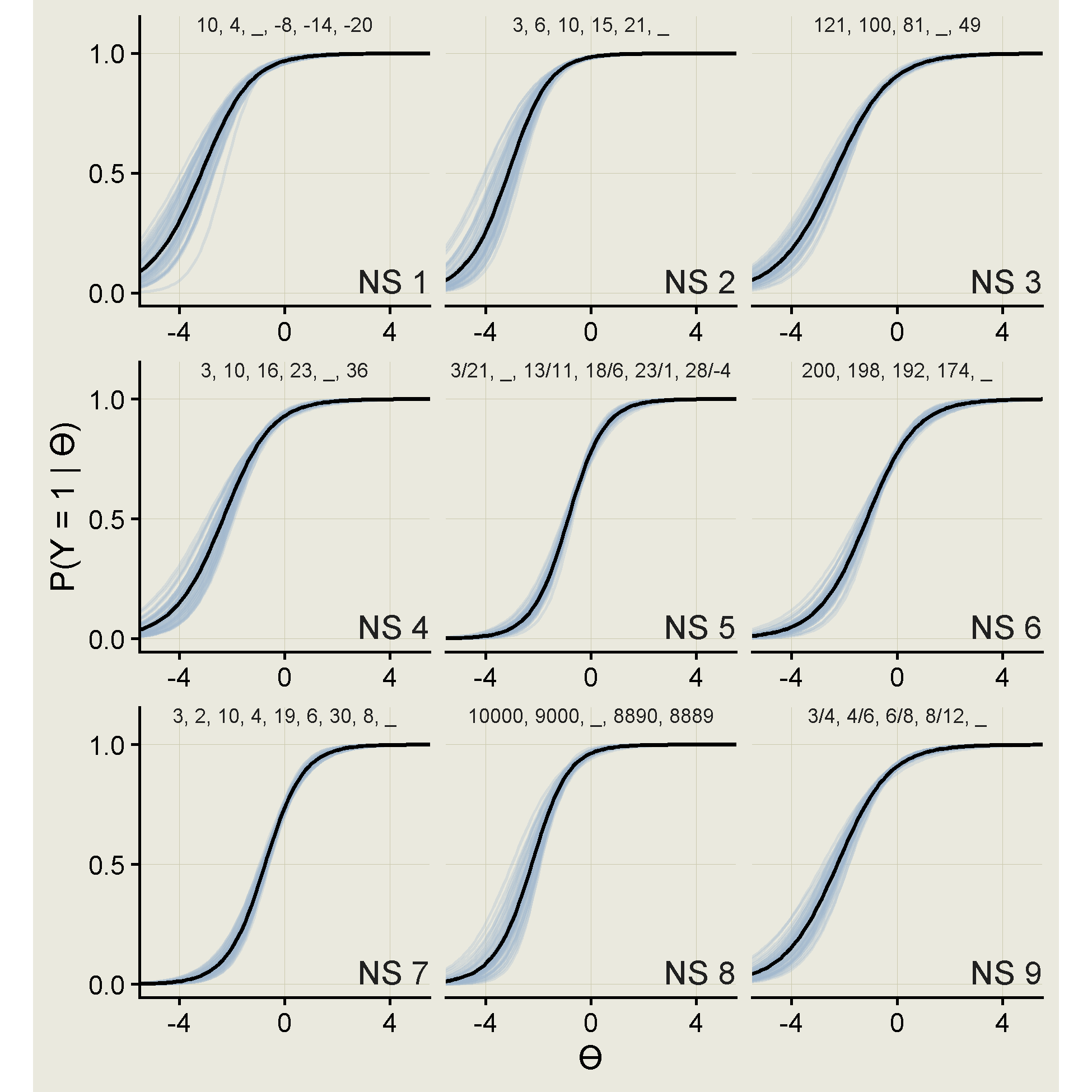
And below are the information curves.
ps |>
  ggplot(aes(x = th, y = info, group = rep)) +
  geom_line(alpha = .3, color = "slategray3") +
  geom_line(data = ps |> summarize(.by = c(th, item),
                                   info = mean(info)),
            aes(x = th, y = info),
            inherit.aes = F, linewidth = .8) +
  geom_text(data = summarize(ps, .by = item), aes(label = glue::glue("NS {item}")),
            x = Inf, y = .05, color = "#202020",
            hjust = 1,
            inherit.aes = F) +
  geom_text(data = ns_labels, aes(label = series),
            x = 0, y = Inf, color = "#202020",
            hjust = 0.5, vjust = 1, size = 3,
            inherit.aes = F) +
  scale_y_continuous(breaks = c(0, 1, 2)) +
  scale_x_continuous(breaks = c(-4, 0, 4)) +
  coord_cartesian(xlim = c(-5, 5), ylim = c(0, 1.5)) +
  facet_wrap(~ fct_inorder(item), nrow = 3, axes = "all_x") +
  labs(y = "I(ϴ)", x = "ϴ") +
  theme_classic(base_size = 14, paper = "#eae9de") +
  theme(strip.background = element_blank(),
        strip.text.x = element_blank(),
        aspect.ratio = 1,
        panel.grid.major = element_line(scales::col_darker("#eae9de", 15), 0.1))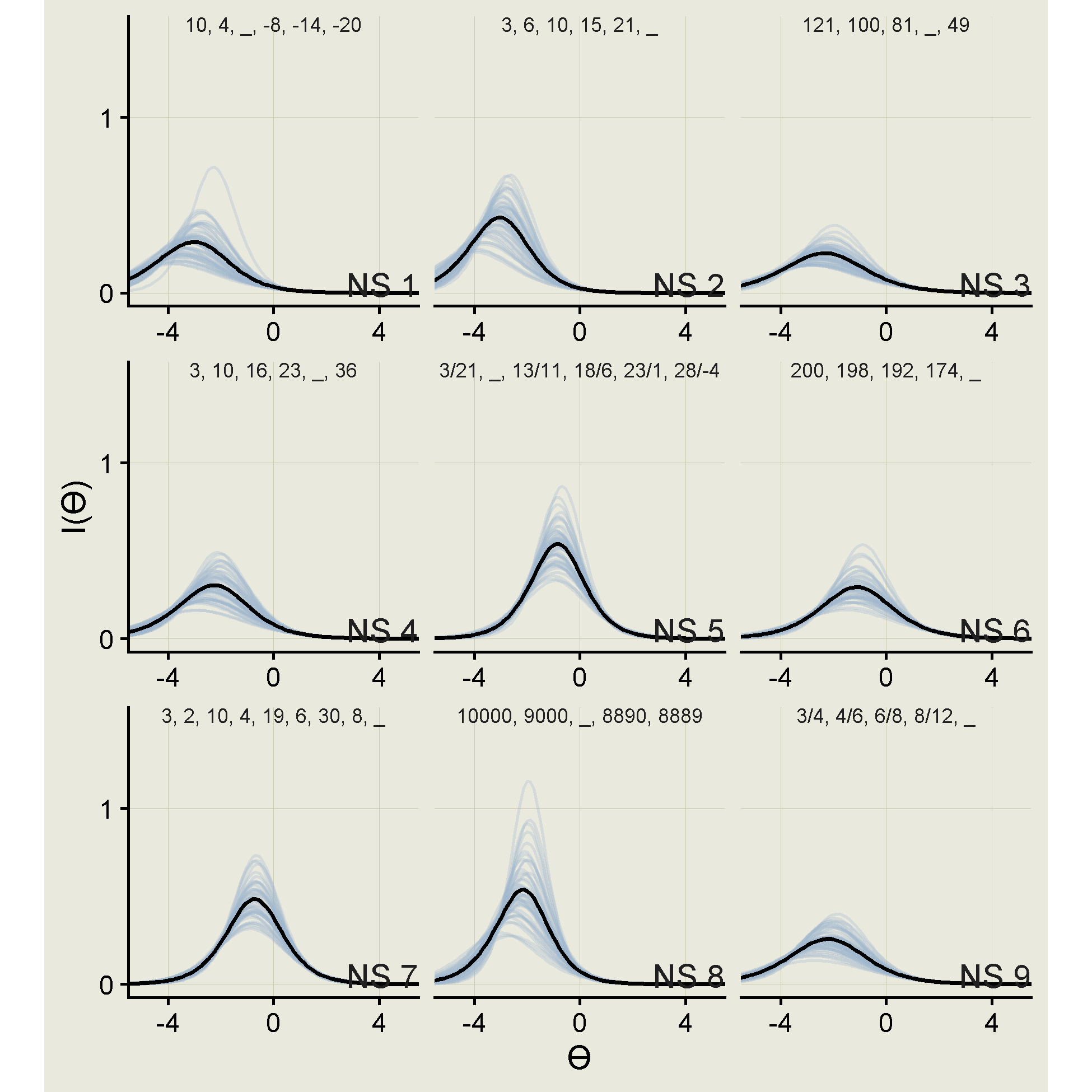
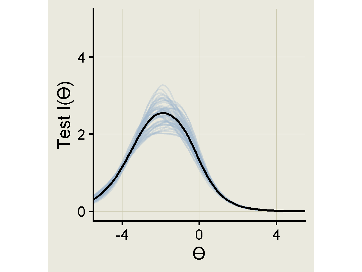
Test information curve
ps |>
  summarize(.by = c(rep, th),
            test_info = sum(info)) |>
  ggplot(aes(x = th, y = test_info, group = rep)) +
  geom_line(alpha = .3, color = "slategray3") +
  geom_line(data = ps |> summarize(.by = c(rep, th),
            test_info = sum(info)) |>
              summarize(.by = th,
                        test_info = mean(test_info)),
            aes(x = th, y = test_info),
            inherit.aes = F, linewidth = .8) +
  scale_y_continuous(breaks = c(0, 2, 4)) +
  scale_x_continuous(breaks = c(-4, 0, 4)) +
  coord_cartesian(xlim = c(-5, 5), ylim = c(0, 5)) +
  labs(y = "Test I(ϴ)", x = "ϴ") +
  theme_classic(base_size = 14, paper = "#eae9de") +
  theme(strip.background = element_blank(),
        aspect.ratio = 1,
        panel.grid.major = element_line(scales::col_darker("#eae9de", 15), 0.1))