Bayesian Update

Setup

library(tidyverse)

Reading

bu_full <- rio::import("https://raw.githubusercontent.com/forecastingresearch/fpt/refs/heads/main/data_cognitive_tasks/task_datasets/data_bayesian_update.csv")

anchoraig_full <- rio::import("https://raw.githubusercontent.com/forecastingresearch/fpt/refs/heads/main/data_cognitive_tasks/metadata_tables/task_aig_version.csv")

dn_dat <- readRDS(here::here("Data", "Denominator Neglect", "dn_dat.rds"))

dn_topitems <- readRDS(here::here("Data", "Denominator Neglect", "top_items.rds"))

Functions

# calculates the correlation between a randomly sample group of `n_items` and s-scores
bu_func <- function(data, n_items, rep = 1:1) {
  pmap(expand_grid(n_items = n_items, rep = rep), 
          \(n_items, rep) {
            
            data |>
              filter(unique_trial %in% sample(unique(unique_trial), n_items)) |>
              
              # get person-level scores for both `sscore` and BU (`score`)
              summarize(.by = subject_id,
                        sscore = first(sscore),
                        score = mean(score),
                        n_items = n()) |>
              select(sscore, score) |>
              drop_na() |>
              summarize(n_items = n_items,
                        rep = rep,
                        cor = cor(sscore, score) |> abs())
          }) |>
    list_rbind()
}

# calculates the R^2 of a linear model with `n_items` BU items and the top five DN items
bu_r2_func <- function(data, n_items, rep = 1) {
  pmap(expand_grid(n_items = n_items, rep = rep), 
       \(n_items, rep) {
         
         data |>
           filter(unique_trial %in% sample(unique(unique_trial), n_items)) |>
           summarize(.by = subject_id,
                     sscore = first(sscore),
                     correct = first(correct),
                     score = mean(score),
                     n_items = n()) |>
           select(sscore, score, correct) |>
           drop_na() |>
           summarize(n_items = n_items,
                     rep = rep,
                     r2 = lm(sscore ~ score + correct,
                             data = data.frame(sscore, score, correct)) |> 
                       summary() |>
                       pluck("r.squared"))
       }) |>
    list_rbind()
}

Cleaning

Easy

anchor_ids_e <- anchoraig_full %>%
  filter(task == "bayesian_update_easy" |
           task == "bayesian_update_hard") %>%
  mutate(task_version = factor(ifelse(task == "bayesian_update_easy", "easy", "hard"))) %>%
  select(!task) %>%
  
  # because participants did more than one version in a session, need to specify both anchor and AIG both here and in the following assignment to get just the specific quadrant
  filter(AIG_version == "anchor" & task_version == "easy") %>%
  pull(session_id)

bu_dat_e <- bu_full %>%
  arrange(session_id, unique_trial) %>%
  
  # only anchor version and only easy version
  filter(session_id %in% anchor_ids_e & version == "easy") |>
  select(session_id, unique_trial, score, ball_split) |>
  left_join(rio::import("https://raw.githubusercontent.com/forecastingresearch/fpt/refs/heads/main/data_cognitive_tasks/metadata_tables/session.csv"),
            by = "session_id") |>
  left_join(rio::import("https://raw.githubusercontent.com/forecastingresearch/fpt/refs/heads/main/data_forecasting/processed_data/scores_quantile.csv") |>
            select(subject_id, sscore_standardized) |>
              
            # mean sscores per person
            summarize(.by = subject_id,
                      sscore = mean(sscore_standardized)),
            by = "subject_id") |>
  select(subject_id, unique_trial, ball_split, score, sscore) |>
  
  # mean score per BU item (over the five trials)
  # suggestion (maybe): do some trial-level stuff at some point?
  summarize(.by = c(subject_id, unique_trial),
            score = mean(score),
            sscore = first(sscore),
            ball_split = first(ball_split))

saveRDS(bu_dat_e, here::here("Data", "Bayesian Update", "bu_dat_e.rds"))

Hard

anchor_ids_h <- anchoraig_full %>%
  filter(task == "bayesian_update_easy" |
           task == "bayesian_update_hard") %>%
  mutate(task_version = factor(ifelse(task == "bayesian_update_easy", "easy", "hard"))) %>%
  select(!task) %>%
  
  # because participants did more than one version in a session, need to specify both anchor and AIG both here and in the following assignment to get just the specific quadrant
  filter(AIG_version == "anchor" & task_version == "hard") %>%
  pull(session_id)

bu_dat_h <- bu_full %>%
  arrange(session_id, unique_trial) %>%
  
  # only anchor version and only easy version
  filter(session_id %in% anchor_ids_h & version == "hard") |>
  select(session_id, unique_trial, score, ball_split) |>
  left_join(rio::import("https://raw.githubusercontent.com/forecastingresearch/fpt/refs/heads/main/data_cognitive_tasks/metadata_tables/session.csv"),
            by = "session_id") |>
  left_join(rio::import("https://raw.githubusercontent.com/forecastingresearch/fpt/refs/heads/main/data_forecasting/processed_data/scores_quantile.csv") |>
            select(subject_id, sscore_standardized) |>
              
            # mean sscores per person
            summarize(.by = subject_id,
                      sscore = mean(sscore_standardized)),
            by = "subject_id") |>
  select(subject_id, unique_trial, ball_split, score, sscore) |>
  
  # mean score per BU item (over the five trials)
  # suggestion (maybe): do some trial-level stuff at some point?
  summarize(.by = c(subject_id, unique_trial),
            score = mean(score),
            sscore = first(sscore),
            ball_split = first(ball_split))

saveRDS(bu_dat_h, here::here("Data", "Bayesian Update", "bu_dat_h.rds"))

library(tidyverse)

bu_full <- rio::import("https://raw.githubusercontent.com/forecastingresearch/fpt/refs/heads/main/data_cognitive_tasks/task_datasets/data_bayesian_update.csv")

anchoraig_full <- rio::import("https://raw.githubusercontent.com/forecastingresearch/fpt/refs/heads/main/data_cognitive_tasks/metadata_tables/task_aig_version.csv")

bu_full |>
  summarize(.by = trial,
            draw = list(unique(current_draw)))

   trial      draw
1      0 blue, red
2      1 blue, red
3      2 blue, red
4      3 blue, red
5      4 blue, red
6      5 red, blue
7      6 red, blue
8      7 blue, red
9      8 red, blue
10     9 blue, red
11    10 red, blue
12    11 red, blue
13    12 red, blue
14    13 red, blue
15    14 red, blue
16    15 red, blue
17    16 red, blue
18    17 red, blue
19    18 blue, red
20    19 blue, red
21    20 blue, red
22    21 red, blue
23    22 blue, red
24    23 blue, red
25    24 red, blue
26    25 red, blue
27    26 red, blue
28    27 blue, red
29    28 red, blue
30    29 red, blue
31    30 red, blue
32    31 red, blue
33    32 blue, red
34    33 red, blue
35    34 red, blue
36    35 red, blue
37    36 red, blue
38    37 blue, red
39    38 red, blue
40    39 red, blue

anchor_ids_h <- anchoraig_full %>%
  filter(task == "bayesian_update_hard" & AIG_version == "anchor") |>
  pull(session_id)

bu_full %>%
  filter(session_id %in% anchor_ids_h & version == "hard") |>
  summarize(.by = trial,
            ball_split = unique(ball_split),
            draw = unique(current_draw))

   trial ball_split draw
1      0      40,60 blue
2      1      40,60 blue
3      2      40,60  red
4      3      40,60 blue
5      4      40,60 blue
6      5      30,70 blue
7      6      30,70  red
8      7      30,70  red
9      8      30,70 blue
10     9      30,70 blue
11    10      40,60  red
12    11      40,60 blue
13    12      40,60 blue
14    13      40,60  red
15    14      40,60 blue
16    15      40,60  red
17    16      40,60 blue
18    17      40,60  red
19    18      40,60  red
20    19      40,60  red
21    20      30,70 blue
22    21      30,70 blue
23    22      30,70  red
24    23      30,70 blue
25    24      30,70 blue
26    25      30,70 blue
27    26      30,70 blue
28    27      30,70  red
29    28      30,70 blue
30    29      30,70 blue
31    30      40,60 blue
32    31      40,60 blue
33    32      40,60 blue
34    33      40,60  red
35    34      40,60  red
36    35      30,70 blue
37    36      30,70  red
38    37      30,70  red
39    38      30,70 blue
40    39      30,70  red

The following analysis only focuses on Bayesian Update: Easy

Correlations Between Bayesian Update and S-Scores

The overall correlation between mean scores on Bayesian Update and s-scores was 0.44.

bu_dat_e |>
  filter(unique_trial %in% sample(unique(unique_trial), 8)) |>
  summarize(.by = subject_id,
            sscore = first(sscore),
            score = mean(score)) |>
  ggplot(aes(x = score, y = sscore)) +
  geom_point() +
  # chore: italicize "r"
  geom_label(label = paste("r =", (bu_dat_e |>
                                       summarize(.by = subject_id, sscore = first(sscore), score = mean(score)) |> 
                                       drop_na() |>
                                       select(sscore, score) |>
                                       cor() |> 
                                      round(2))[1, 2]),
             x = Inf, y = Inf, hjust = 1, vjust = 1) +
  labs(y = "S-Score", x = "Bayesian Update") +
  guides(x = guide_axis(cap = "both"), y = guide_axis(cap = "both")) +
  theme_classic() +
  theme(aspect.ratio = 1)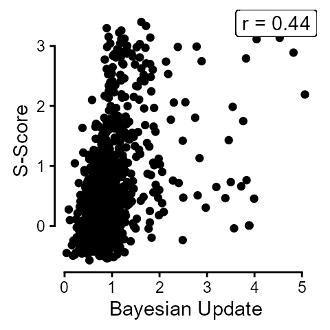

We randomly selected \(n\) items where \(n \in [1, 8]\) and calculated the correlations between person-level mean scores on those \(n\) items and s-scores, doing 100 replications per \(n\).

bu_cors <- bu_func(bu_dat_e, 1:8, 1:100)
saveRDS(bu_cors, here::here("Data", "Bayesian Update", "bu_cors.rds"))

bu_cors <- readRDS(here::here("Data", "Bayesian Update", "bu_cors.rds"))

bu_cors |>
    summarize(.by = c(n_items),
            across(cor, list(mean = mean,
                             lower = ~ quantile(.x, 0.05, names = FALSE),
                             upper = ~ quantile(.x, 0.95, names = FALSE)))) |>
  ggplot(aes(x = n_items, y = cor_mean)) +
  geom_line(linewidth = 1.5, color = "slategray") +
  geom_ribbon(aes(ymin = cor_lower, ymax = cor_upper),
              alpha = .3, fill = "slategray") +
  scale_x_continuous(breaks = c(1, 3, 6, 8)) +
  scale_y_continuous(breaks = c(.2, .4, .6)) +
  coord_cartesian(ylim = c(.2, .6)) +
  labs(y = "Correlation with S-Score", x = "Number of Items") +
  guides(x = guide_axis(cap = "both"), y = guide_axis(cap = "both")) +
  theme_classic()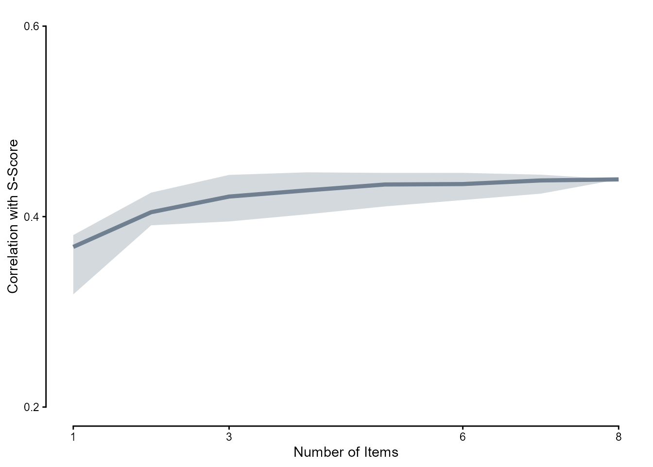 

Correlations Between Bayesian Update and S-Score Residuals

We first residualized out the effect of the top five Denominator Neglect items.

dn_topfive <- dn_topitems |>
  pivot_longer(c(conf_item, harm_item),
               names_to = "choice_type", values_to = "item") |>
  filter(rank <= 5) |>
  pull(item)

dn_topfivedat <- dn_dat |> 
  filter(item %in% dn_topfive) |> 
  summarize(.by = subject_id,
            sscore = first(sscore),
            correct = mean(correct)) |> # alert alert
  drop_na()

dn_resids <- data.frame(subject_id = dn_topfivedat$subject_id,
      residuals = lm(sscore ~ correct, data = dn_topfivedat)$residuals)

The overall correlation between mean scores on Bayesian Update and s-score residuals was 0.29.

bu_dat_e |>
  left_join(dn_resids, by = "subject_id") |>
  mutate(sscore = residuals) |>
  summarize(.by = subject_id,
            sscore = first(sscore),
            score = mean(score)) |>
  ggplot(aes(x = score, y = sscore)) +
  geom_point() +
  # chore: italicize "r"
  geom_label(label = paste("r =", (bu_dat_e |>
  left_join(dn_resids, by = "subject_id") |>
  mutate(sscore = residuals) |>
                                       summarize(.by = subject_id, sscore = first(sscore), score = mean(score)) |> 
                                       drop_na() |>
                                       select(sscore, score) |>
                                       cor() |> 
                                      round(2))[1, 2]),
             x = Inf, y = Inf, hjust = 1, vjust = 1) +
  labs(y = "S-Score Residuals", x = "Bayesian Update") +
  guides(x = guide_axis(cap = "both"), y = guide_axis(cap = "both")) +
  theme_classic() +
  theme(aspect.ratio = 1)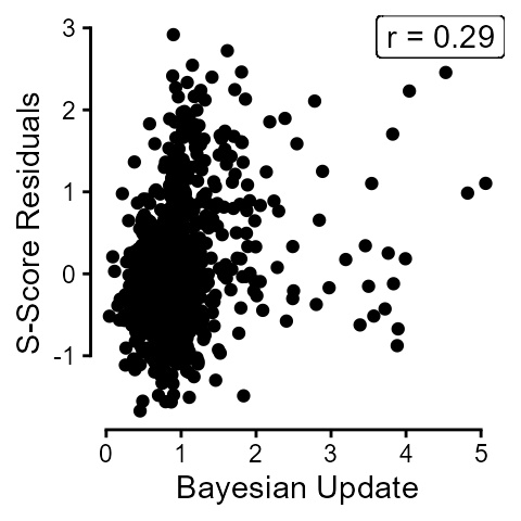

bu_cors_postdn <- bu_dat_e |>
  left_join(dn_resids, 
            by = "subject_id") |>
  mutate(sscore = residuals) |>
  bu_func(1:8, 1:100)

saveRDS(bu_cors_postdn, here::here("Data", "Bayesian Update", "bu_cors_postdn.rds"))

bu_cors_postdn <- readRDS(here::here("Data", "Bayesian Update", "bu_cors_postdn.rds"))

bu_cors_postdn |>
  summarize(.by = c(n_items),
            across(cor, list(mean = mean,
                             lower = ~ quantile(.x, 0.05, names = FALSE),
                             upper = ~ quantile(.x, 0.95, names = FALSE)))) |>
  ggplot(aes(x = n_items, y = cor_mean)) +
  geom_line(linewidth = 1.5, color = "slategray") +
  geom_ribbon(aes(ymin = cor_lower, ymax = cor_upper),
              alpha = .3, fill = "slategray") +
  scale_x_continuous(breaks = c(1, 3, 6, 8)) +
  scale_y_continuous(breaks = c(.2, .3, .4)) +
  coord_cartesian(ylim = c(.2, .4)) +
  labs(y = "Correlation with S-Score Residuals", x = "Number of Items",
       caption = "Top five Denominator Neglect items\nresidualized out of s-scores") +
  guides(x = guide_axis(cap = "both"), y = guide_axis(cap = "both")) +
  theme_classic()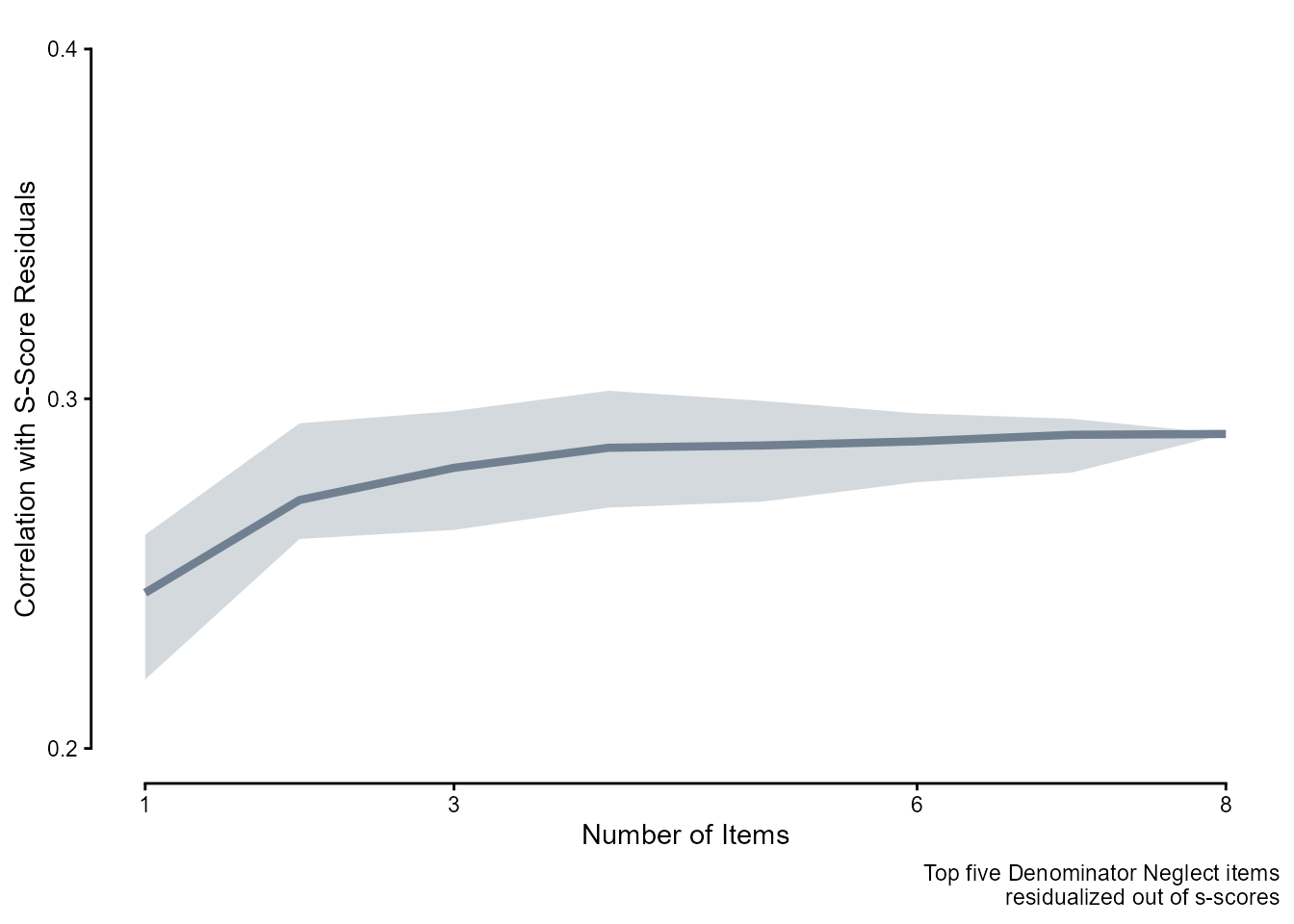 

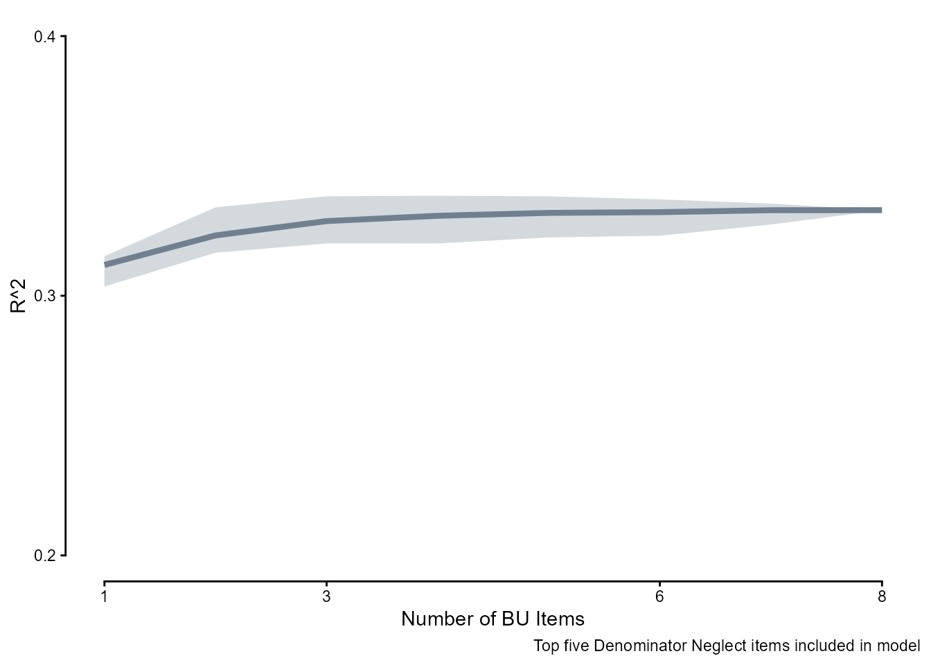
\(R^2\) Post-DN and BN

To see how successful the combinations of the five Denominator Neglect items and \(n\) Bayesian Update items are at capturing forecasting ability, here is the \(R^2\) of a simple linear model with increasing \(n\) of Bayesian Update items in the person-level means scores.

bu_r2 <- bu_dat_e |>
           left_join(dn_topfivedat,
                     by = c("subject_id", "sscore")) |>
  bu_r2_func(1:8, 1:100)

saveRDS(bu_r2, here::here("Data", "Bayesian Update", "bu_r2.rds"))

bu_r2 <- readRDS(here::here("Data", "Bayesian Update", "bu_r2.rds"))

bu_r2 |>
  summarize(.by = c(n_items),
            across(r2, list(mean = mean,
                             lower = ~ quantile(.x, 0.05, names = FALSE),
                             upper = ~ quantile(.x, 0.95, names = FALSE)))) |>
  ggplot(aes(x = n_items, y = r2_mean)) +
  geom_line(linewidth = 1.5, color = "slategray") +
  geom_ribbon(aes(ymin = r2_lower, ymax = r2_upper),
              alpha = .3, fill = "slategray") +
  scale_x_continuous(breaks = c(1, 3, 6, 8)) +
  scale_y_continuous(breaks = c(.2, .3, .4)) +
  coord_cartesian(ylim = c(.2, .4)) +
  labs(y = "R^2", x = "Number of BU Items",
       caption = "Top five Denominator Neglect items included in model") +
  guides(x = guide_axis(cap = "both"), y = guide_axis(cap = "both")) +
  theme_classic()