2PL

library(tidyverse)

2PL Modeling Strategy

Included: Denominator Neglect, Decision Rules

\[ logodds(P(Y = 1)) = a (\theta - b) \], where \(b\) represents the item’s difficulty and \(a\) represents the item’s discrimination.

Difficulty corresponds to the location of the item response curve, indicating how… difficult… the item is to get correct. Higher difficulty corresponds to harder items, and difficulty values scale with \(\theta\): an item with a difficultly value of \(b = 0\) means that an examinee with average skill \(\theta = 0\) would have a 50% chance of a correct answer.

Discrimination corresponds to the steepness of the item response curve and indicates how well items… discriminate… among \(\theta\) levels. Higher values indicate steeper slopes which better discriminate among skill levels.

expand_grid(a = c(.5, 1, 1.5),
            b = c(-2, 0, 2),
            theta = seq(-5, 5, length.out = 100)) |>
  mutate(p = plogis(a * (theta - b))) |>
  ggplot(aes(x = theta, y = p)) +
  geom_line() +
  scale_x_continuous(breaks = c(-3, 0, 3)) +
  scale_y_continuous(breaks = c(0, .5, 1)) +
  guides(x = guide_axis(cap = "both"),
         y = guide_axis(cap = "both")) +
  facet_grid(cols = vars(a), rows = vars(b),
             labeller = label_both,
            axes = "all") +
  theme_classic() +
  theme(strip.background = element_blank())

2PL Stan Code

Parameter Estimates to Curves

To get item response and information curves from the Stan model’s parameter estimates, we first converted the item paramter estimates to probabilites of a correct answer for a range of theoretical \(\theta\) values.

\[ P(Y = 1 | \theta) \bigg|_{\theta \in [-5, 5]} = \frac{e^{\hat{a} (\theta - \hat{b})}}{1 + e^{\hat{a} (\theta - \hat{b})}} \]

dat <- expand_grid(a = c(.5, 1, 1.5),
            b = c(-2, 0, 2),
            theta = seq(-5, 5, length.out = 100)) |>
  mutate(p = plogis(a * (theta - b)))

We plotted those predicted probabilities of a correct answer for the theoretical \(\theta\) values.

dat |>
  ggplot(aes(x = theta, y = p)) +
  geom_line() +
  scale_x_continuous(breaks = c(-3, 0, 3)) +
  scale_y_continuous(breaks = c(0, .5, 1)) +
  guides(x = guide_axis(cap = "both"),
         y = guide_axis(cap = "both")) +
  facet_grid(cols = vars(a), rows = vars(b),
             labeller = label_both,
            axes = "all") +
  theme_classic() +
  theme(strip.background = element_blank())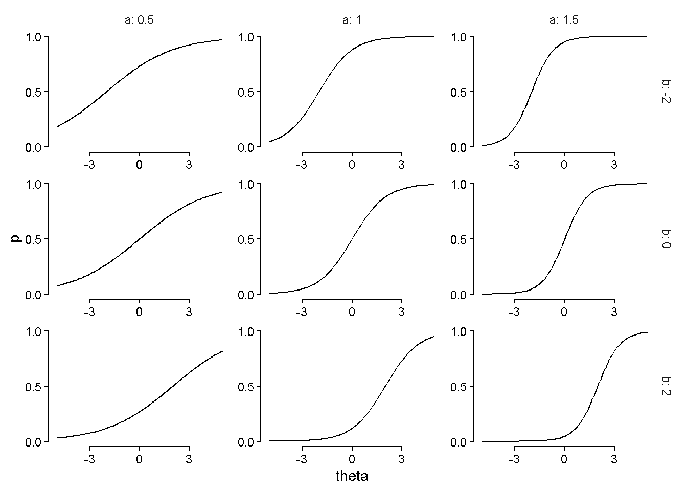

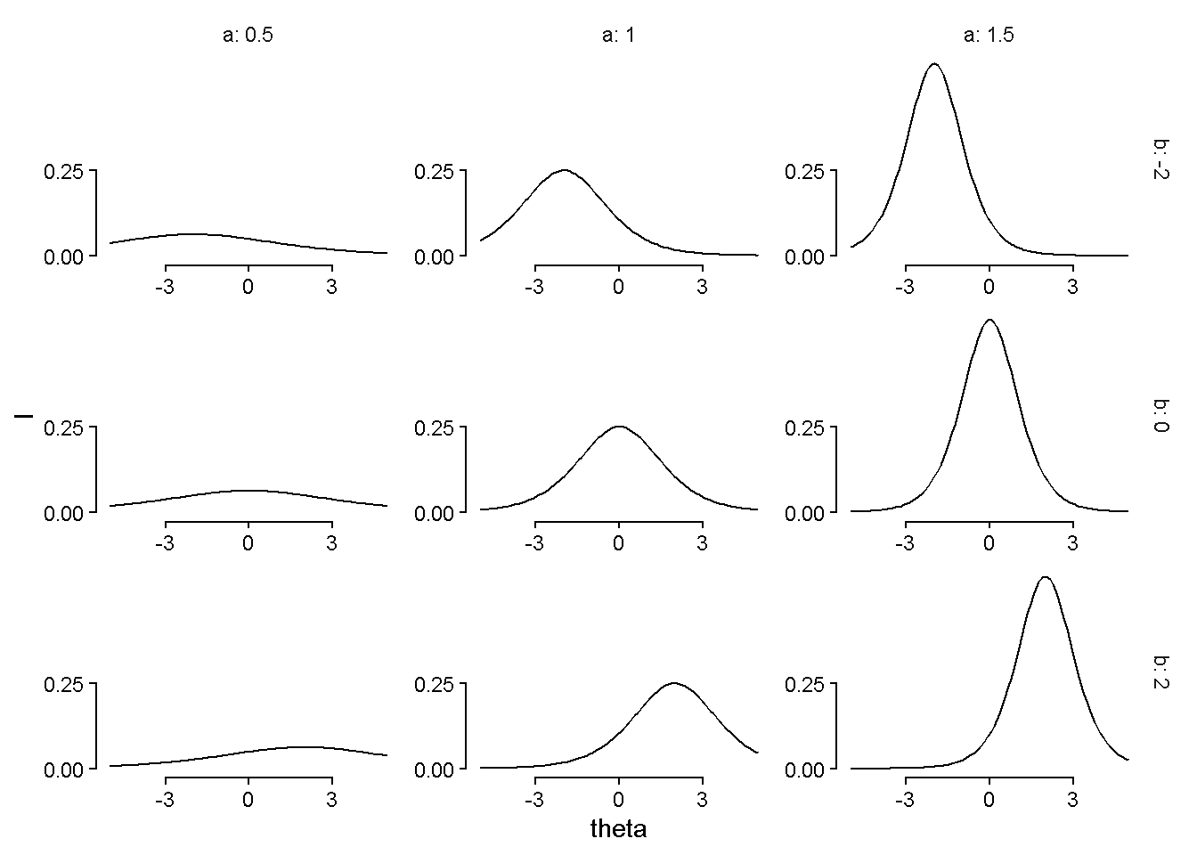
To get information curves for an item, we multiply the probability of a correct answer by the probability of an incorrect answer and by the square of the discrimination parameter.

\[ I(\theta) \bigg|_{\theta \in [-5, 5]} = a^2 \times P(Y = 1) \times P(Y = 0) = a^2 \times P(Y = 1) \times (1 - P(Y = 1)) \]

And plot the information function values over theoretical values of \(\theta\).

dat |>
  mutate(I = a^2 * p * (1 - p)) |>
  ggplot(aes(x = theta, y = I)) +
  geom_line() +
  scale_x_continuous(breaks = c(-3, 0, 3)) +
  scale_y_continuous(breaks = c(0, .25)) +
  guides(x = guide_axis(cap = "both"),
         y = guide_axis(cap = "both")) +
  facet_grid(cols = vars(a), rows = vars(b),
             labeller = label_both,
            axes = "all") +
  theme_classic() +
  theme(strip.background = element_blank())