Chi-Squared Test

PSYC 2020-A01 / PSYC 6022-A01 | 2025-11-07 | Lab 12

Jessica Helmer

Outline

Chi-Squared (\(\chi^2\)) Test

Learning objectives:

R: \(\chi^2\) Tests

Chi-Squared (\(\chi^2\)) Test

Testing inferences about proportions

○ Involve categorical variables

Comparing observed frequencies (counts) to some expected (null hypothesis) frequencies

\(\chi^2\) Test of Goodness of Fit: expected frequencies are set by researcher (e.g., null hypothesis is equal frequencies across all groups)

\(\chi^2\) Test of Independence: expected frequencies are those implied by independence

Chi-Squared (\(\chi^2\)) Test

Instead of a continuous variable, our outcome is a count

Continuous

Height
Petal length
Test score

Counts

Coin flip being heads
Number of pets
Goals scored

Only integers

\(\chi^2\) Test of Goodness of Fit

Do the observed frequencies of a categorical variable differ from what expected a priori?

Typically, this expectation is equal occurrence across groups (but doesn’t have to be).

If equal occurrence, what would be our expected frequencies?

100 coin flips

Heads	Tails
50	50

Favorite primary color of 33 students

Red	Blue	Yellow
11	11	11

Can also hypothesize proportions and convert to frequencies once you have a sample size.

\(\chi^2\) Test of Goodness of Fit: Hypotheses

\(H_0\): Observed data match the expected frequencies for the population

\(H_1\): Observed data do not match the expected frequencies for the population

○ Observed frequency is significantly different than expected

\(H_0\): \(\pi_j = \pi_{j_0}\) for all categories \(j\) (i.e., difference for all categories is 0), where

\(\pi_j\) = observed proportion

\(\pi_{j_0}\) = expected proportion

\(H_1\): \(\pi_j \neq \pi_{j_0}\) for any category \(j\)

\(\chi^2\) Test of Goodness of Fit Generally

\[ \chi^2 = \sum_{j=1}^{J} \frac{(O_j – N\pi_{j_0})^2}{N\pi_{j_0}} = \sum_{j=1}^{J} \frac{(O_j – E_j)^2}{E_j} \]

where

\(O_j\) = observed frequency

\(N\) = total sample size

\(E_j\) = expected frequency

\(j\) = individual category out of \(J\) total categories

The sum of the squared differences between the observed and expected frequencies, divided by the expected frequency, for each group.

\(\chi^2\) Test of Goodness of Fit Generally

\(\text{df} = J - 1\), where

\(J\) = number of categories

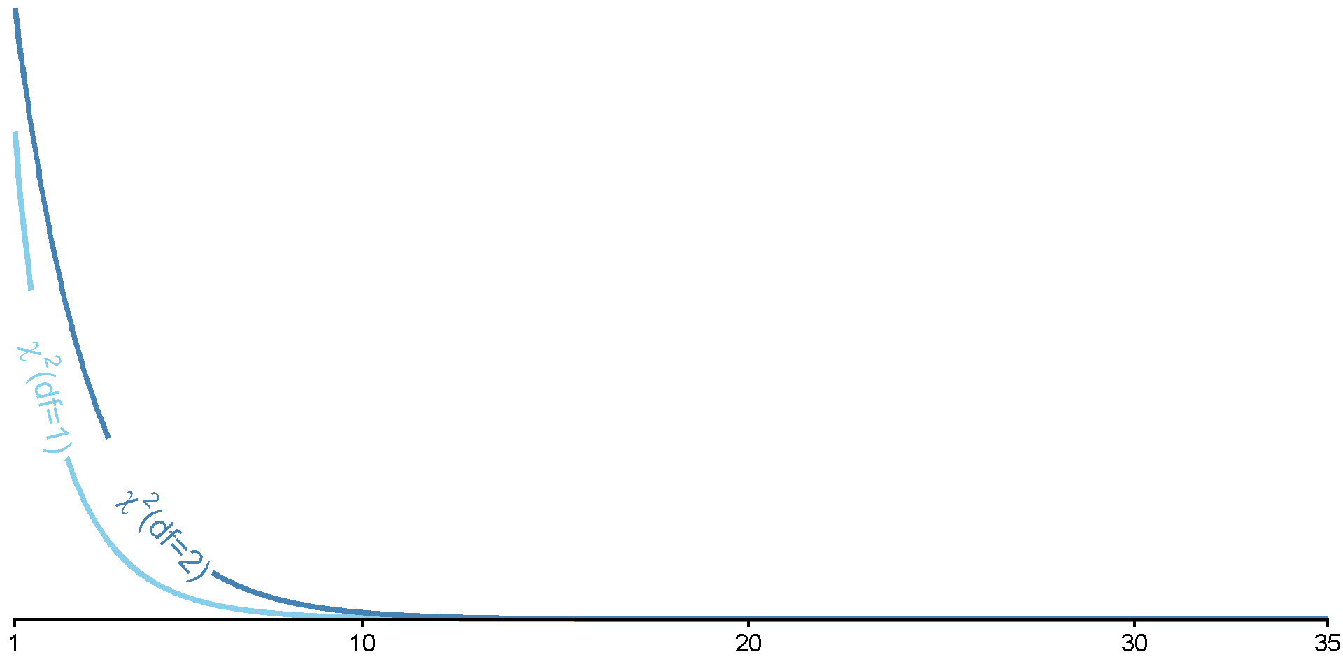
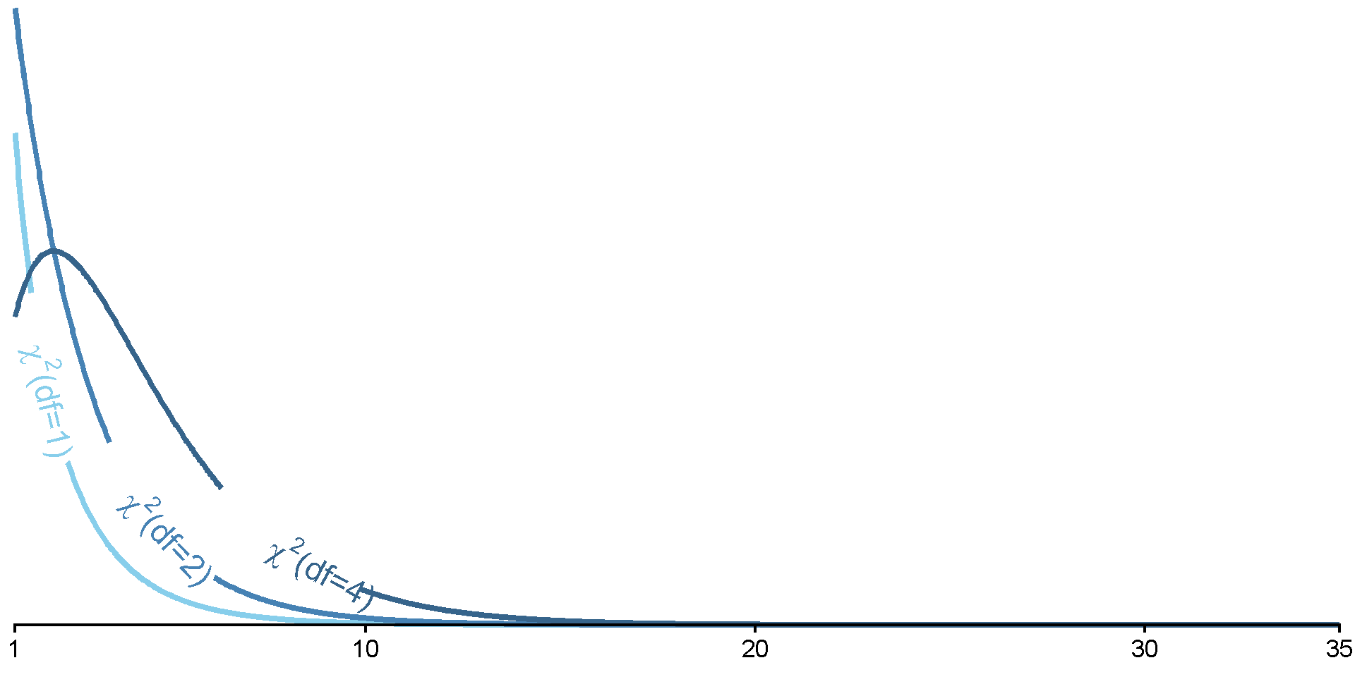
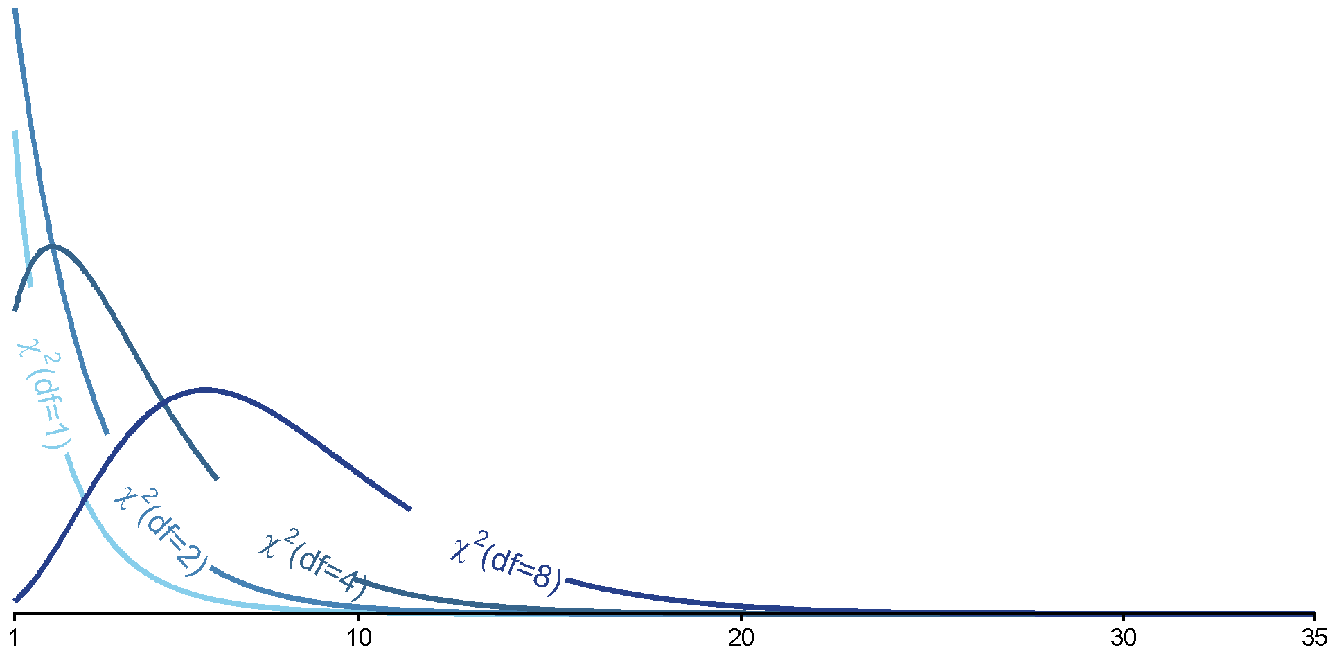
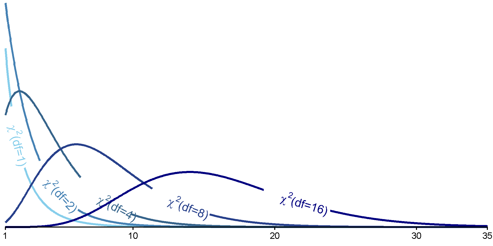
Use to identify critical \(\chi^2\) value from \(\chi^2\) table, R, etc.

For \(\chi^2\), as \(\text{df}\) increases, so does the critical-\(\chi^2\) value (at same \(\alpha\))

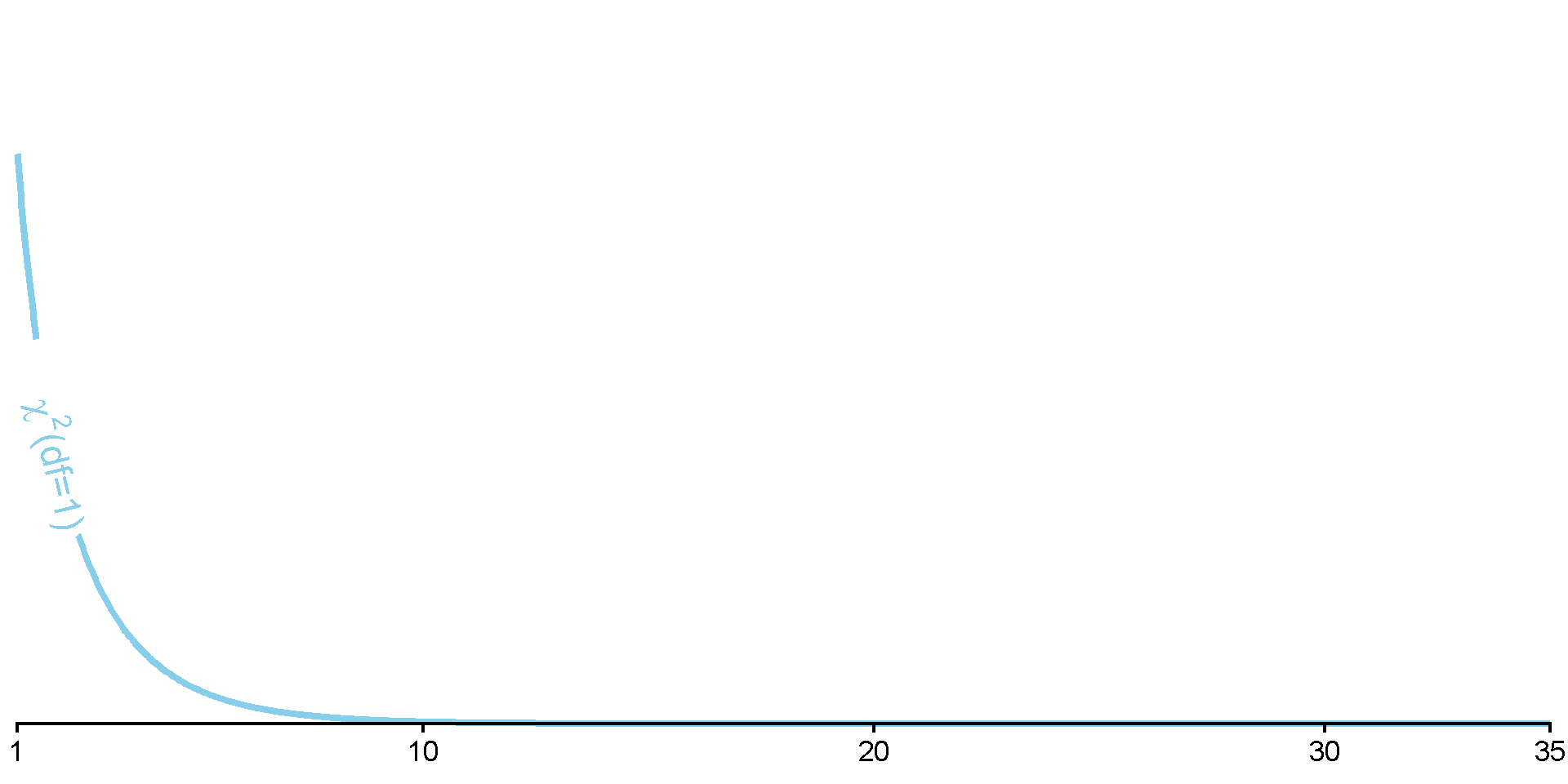
Only ever a one-tailed test! For the upper end of the distribution.

\(\chi^2\) Distribution

\(\chi^2\) Test of Goodness of Fit Cutoffs

Cutoff for test of heads vs. tails

\(J =\) 2

\(\text{df} = J - 1 =\) 1

qchisq(.95, 1)

[1] 3.841459

qchisq(.05, 1, lower.tail = F)

[1] 3.841459

Cutoff for test of favorite color in the rainbow

\(J =\) 7 (ROYGBIV)

\(\text{df} = J - 1 =\) 6

qchisq(.95, 6)

[1] 12.59159

qchisq(.05, 6, lower.tail = F)

[1] 12.59159

\(\chi^2\) Test of Goodness of Fit Example

You are an education psychologist interested in college students’ choice of majors. You’ve grouped majors into five categories: STEM, Social Sciences, Humanities, Arts, and Business. You’d like to test whether there are differences in the population of students choosing those majors. You sample 100 students and ask what major they chose.

First, what are your expected frequencies for each category?

	STEM	Social Sciences	Humanities	Arts	Business
Expected
Observed

\(\chi^2\) Test of Goodness of Fit Example

First, what are your expected frequencies for each category?

	STEM	Social Sciences	Humanities	Arts	Business
Expected	20	20	20	20	20
Observed

\(\chi^2\) Test of Goodness of Fit Example

Next, what is your \(\chi^2\) cutoff value?

	STEM	Social Sciences	Humanities	Arts	Business
Expected	20	20	20	20	20
Observed

\(\chi^2\) Test of Goodness of Fit Example

Cutoff in R

df <- 5 - 1
chisq_crit <- qchisq(.95, df)
chisq_crit

[1] 9.487729

\(\chi^2\) Test of Goodness of Fit Example

Here are the observed values:

	STEM	Social Sciences	Humanities	Arts	Business
Expected	20	20	20	20	20
Observed	65	10	5	5	15

\(\chi^2\) Test of Goodness of Fit Example

\[ \chi^2 = \sum_{j=0}^{J} \frac{(O_j – N\pi_j)^2}{N\pi_j} = \sum_{j=0}^{J} \frac{(O_j – E_j)^2}{E_j} \]

obs_chisq <- (65 - 20)^2 / 20 +
  (10 - 20)^2 / 20 +
  (5 - 20)^2 / 20 +
  (5 - 20)^2 / 20 +
  (15 - 20)^2 / 20
obs_chisq

[1] 130

obs_chisq > chisq_crit

[1] TRUE

We can reject the null in favor of the alternative that the number of students is not the same across majors.

\(\chi^2\) Test of Goodness of Fit R Function

majordat <- data.frame(major = c("STEM", "Social.Sciences", "Humanities", "Arts", "Business"),
           observed = c(65, 10, 5, 5, 15))

chisq <- majordat |>
  select(observed) |>
  chisq.test()
chisq


    Chi-squared test for given probabilities

data:  select(majordat, observed)
X-squared = 130, df = 4, p-value < 2.2e-16

chisq$expected

[1] 20 20 20 20 20

chisq$statistic

X-squared 
      130

chisq$p.value

[1] 3.89406e-27

\(\chi^2\) Test of Goodness of Fit Example

Let’s restart and say that you were a educational psychologist interested in how students in STEM schools choose their major. In this situation, you had expected more students to select a STEM major than other majors.

These are your new expected frequencies (60% STEM, evenly divided across the rest):

	STEM	Social Sciences	Humanities	Arts	Business
Expected	60	10	10	10	10
Observed	65	10	5	5	15

\(\chi^2\) Test of Goodness of Fit R Function

chisq.test(x = c(65, 10, 5, 5, 15),
           p = c(60, 10, 10, 10, 10),
           rescale.p = T)


    Chi-squared test for given probabilities

data:  c(65, 10, 5, 5, 15)
X-squared = 7.9167, df = 4, p-value = 0.09468

chisq.test(x = c(65, 10, 5, 5, 15),
           p = c(.60, .10, .10, .10, .10))


    Chi-squared test for given probabilities

data:  c(65, 10, 5, 5, 15)
X-squared = 7.9167, df = 4, p-value = 0.09468

○ x = data of frequencies

○ p = expected probabilities

○ rescale.p = [T/F], will rescale p to probabilities if you prefer to input frequencies

\(\chi^2\) Test of Independence

Do the observed frequencies of a categorical variable differ from what expected via properties of independence?

○ Now considering more than one type of category

○ E.g., Number of pets by cat vs. dog people and undergrad vs. post-graduate

	Cat Person	Dog Person
Undergrad
Post-Graduate

Expected frequencies calculated from the marginal totals of the contingency table

○ Expected values determined from data

\(\chi^2\) Test of Independence: Hypotheses

\(H_0\): Categorical Variable 1 and Categorical Variable 2 are independent (i.e., have no association)

\(H_1\): Categorical Variable 1 and Categorical Variable 2 are not independent (i.e., have some association)

○ Do expected frequencies match those expected via independence?

Mathematically the same as before:

\(H_0\): \(\pi_j = \pi_{j_0}\) for all categories \(j\); difference for all categories is 0, where

\(\pi_j\) = observed proportion

\(\pi_{j_0}\) = expected proportion

\(H_1\): \(\pi_j \neq \pi_{j_0}\) for any category \(j\)

Just changing the expected frequencies

\(\chi^2\) Test of Independence Generally

\[ \chi^2 = \sum_{j_1=1}^{J_1}\sum_{j_2=1}^{J_2} \frac{(O_j – N\pi_{j_0})^2}{N\pi_{j_0}} = \sum_{j_1=1}^{J_1}\sum_{j_2=1}^{J_2} \frac{(O_j – E_j)^2}{E_j} \]

Basically identical formula to calculate the \(\chi^2\).

The difference is that our expected frequencies \(E_j\) are derived from the data. Just like before, we calculate the difference from each cell, but now we have two categories that make up the cell.

The sum of the squared differences between the observed and expected frequencies, divided by the expected frequency, for each cell.

\(\chi^2\) Test of Independence Cutoffs

What is the critical \(\chi^2\) value in a test of independence for a 3x2?

\(\text{df} = (J_1 - 1) \times (J_2 - 1)\) or

\(\text{df} = (n_{rows} - 1) \times (n_{cols} - 1)\)

df <- (3 - 1) * (2 - 1)
df

[1] 2

qchisq(.95, df)

[1] 5.991465

\(\chi^2\) Test of Independence Example

You are another educational psychologist, and you’re interested in examining your department’s student body makeup. You wonder whether there is an association between students’ level (graduate vs. undergraduate) and whether they are an in-state student or not. You sample 50 students from your department, and these are the frequencies you observe.

	In-State	Out-of-State
Undergrad	25	10
Graduate	5	10

First, what are your expected frequencies for each category?

\(\chi^2\) Test of Independence Example: Calculating Expected Frequencies

First, get the marginal totals for each column

	In-State	Out-of-State
Undergrad	25	10
Graduate	5	10
Total

\(\chi^2\) Test of Independence Example: Calculating Expected Frequencies

First, get the marginal totals for each column

	In-State	Out-of-State	Total
Undergrad	25	10	35
Graduate	5	10	15
Total	30	20	50

\(\chi^2\) Test of Independence Example: Calculating Expected Frequencies

	In-State	Out-of-State	Total
Undergrad	25	10	35
Graduate	5	10	15
Total	30	20	50

	In-State	Out-of-State	Total
Undergrad	21	14	35
Graduate	9	6	15
Total	30	20	50

Expected cell frequency = \(E_j\) = \(\frac{\text{column total} \times \text{row total}}{N}\)

○ Undergrad & In-State = \(\frac{35 \times 30}{50} = 21\)

○ Undergrad & Out-of-State = \(\frac{35 \times 20}{50} = 14\)

○ Graduate & In-State = \(\frac{15 \times 30}{50} = 9\)

○ Graduate & Out-of-State = \(\frac{15 \times 20}{50} = 6\)

\(\chi^2\) Test of Goodness of Fit Example

\[ \chi^2 = \sum_{j=0}^{J} \frac{(O_j – N\pi_j)^2}{N\pi_j} = \sum_{j=0}^{J} \frac{(O_j – E_j)^2}{E_j} \]

data.frame(type = c("Undergrad", "Graduate", "Total"),
           `In-State` = c(25, 5, 30),
           `Out-of-State` = c(10, 10, 20),
           Total = c(35, 15, 50))

       type In.State Out.of.State Total
1 Undergrad       25           10    35
2  Graduate        5           10    15
3     Total       30           20    50

chisq_crit <- qchisq(.95, df = (2 - 1) * (2 - 1))
chisq_crit

[1] 3.841459

obs_chisq <- (25 - 21)^2 / 21 +
  (10 - 14)^2 / 14 +
  (5 - 9)^2 / 9 +
  (10 - 6)^2 / 6
obs_chisq

[1] 6.349206

obs_chisq > chisq_crit

[1] TRUE

\(\chi^2\) Test of Independence R Function

studdat <- data.frame(type = c("Undergrad", "Graduate"),
           `In-State` = c(25, 5),
           `Out-of-State` = c(10, 10))
studdat |>
  select(-type) |>
  chisq.test(correct = F)


    Pearson's Chi-squared test

data:  select(studdat, -type)
X-squared = 6.3492, df = 1, p-value = 0.01174

○ correct = [T/F], applies a “continuity correction” to the \(\chi^2\) value. Default is T. Change to F!

We can reject the null in favor of the alternative that students’ level (graduate vs. undergraduate) and whether they are an in-state student or not are not independent.

Count Data

Working With Count Data

dat |> head(12)

   student           major            type
1        1            STEM Non-STEM School
2        2      Humanities     STEM School
3        3      Humanities     STEM School
4        4 Social Sciences Non-STEM School
5        5      Humanities     STEM School
6        6            Arts Non-STEM School
7        7 Social Sciences     STEM School
8        8 Social Sciences     STEM School
9        9            STEM     STEM School
10      10            STEM     STEM School
11      11        Business     STEM School
12      12 Social Sciences     STEM School

Working With Count Data: `table()`

Some ways to generate frequencies from categorical variables

table(dat$major)


           Arts        Business      Humanities Social Sciences            STEM 
             23              13              22              19              23

table(dat$major) |>
  data.frame()

             Var1 Freq
1            Arts   23
2        Business   13
3      Humanities   22
4 Social Sciences   19
5            STEM   23

Working With Count Data: `table()`

table(dat$major, dat$type)

                 
                  Non-STEM School STEM School
  Arts                         13          10
  Business                      4           9
  Humanities                   10          12
  Social Sciences              10           9
  STEM                         16           7

table(dat$major, dat$type) |>
  data.frame()

              Var1            Var2 Freq
1             Arts Non-STEM School   13
2         Business Non-STEM School    4
3       Humanities Non-STEM School   10
4  Social Sciences Non-STEM School   10
5             STEM Non-STEM School   16
6             Arts     STEM School   10
7         Business     STEM School    9
8       Humanities     STEM School   12
9  Social Sciences     STEM School    9
10            STEM     STEM School    7

Working With Count Data: `summarize()`

Some ways to generate frequencies from categorical variables

dat |>
  summarize(.by = c(major, type),
            n = n())

             major            type  n
1             STEM Non-STEM School 16
2       Humanities     STEM School 12
3  Social Sciences Non-STEM School 10
4             Arts Non-STEM School 13
5  Social Sciences     STEM School  9
6             STEM     STEM School  7
7         Business     STEM School  9
8       Humanities Non-STEM School 10
9             Arts     STEM School 10
10        Business Non-STEM School  4

dat |>
  summarize(.by = c(major, type),
            n = n()) |>
  arrange(major, type)

             major            type  n
1             Arts Non-STEM School 13
2             Arts     STEM School 10
3         Business Non-STEM School  4
4         Business     STEM School  9
5       Humanities Non-STEM School 10
6       Humanities     STEM School 12
7             STEM Non-STEM School 16
8             STEM     STEM School  7
9  Social Sciences Non-STEM School 10
10 Social Sciences     STEM School  9

Working With Count Data: `count()`

count(x, grouping_var1, grouping_var2, etc.)

○ x = dataframe

○ grouping_vars = variable names to group by

Basically shorthand for:

df |>
  summarise(.by = c(a, b),
            n = n())

Also seems to arrange by default

Working With Count Data: `count()`

count(x, grouping_var1, grouping_var2, etc.)

○ x = dataframe

○ grouping_vars = variable names to group by

dat |>
  summarize(.by = c(major, type),
            n = n())

             major            type  n
1             STEM Non-STEM School 16
2       Humanities     STEM School 12
3  Social Sciences Non-STEM School 10
4             Arts Non-STEM School 13
5  Social Sciences     STEM School  9
6             STEM     STEM School  7
7         Business     STEM School  9
8       Humanities Non-STEM School 10
9             Arts     STEM School 10
10        Business Non-STEM School  4

dat |>
  count(major, type)

             major            type  n
1             Arts Non-STEM School 13
2             Arts     STEM School 10
3         Business Non-STEM School  4
4         Business     STEM School  9
5       Humanities Non-STEM School 10
6       Humanities     STEM School 12
7             STEM Non-STEM School 16
8             STEM     STEM School  7
9  Social Sciences Non-STEM School 10
10 Social Sciences     STEM School  9

Working With Count Data: `summarize()`

If going to put into the chisq.test() function, want to pivot and get rid of additional columns.

Many ways to do this, but one example:

chisqdat <- dat |>
  count(major, type) |>
  pivot_wider(names_from = type,
              values_from = n) |>
  select(-major)
chisqdat

# A tibble: 5 × 2
  `Non-STEM School` `STEM School`
              <int>         <int>
1                13            10
2                 4             9
3                10            12
4                16             7
5                10             9

chisq.test(chisqdat, correct = F)


    Pearson's Chi-squared test

data:  chisqdat
X-squared = 5.7312, df = 4, p-value = 0.2201

dat |>
  ggplot(aes(x = major)) +
  geom_bar() +
  theme_classic(base_size = 14)

Working With Count Data: `geom_bar()`

Plot
Code

dat |>
  ggplot(aes(x = major, fill = type)) +
  geom_bar(position = "dodge") +
  theme_classic(base_size = 14)

Chi-Squared Test

Outline

Chi-Squared (\(\chi^2\)) Test

Chi-Squared (\(\chi^2\)) Test

\(\chi^2\) Test of Goodness of Fit

\(\chi^2\) Test of Goodness of Fit

\(\chi^2\) Test of Goodness of Fit: Hypotheses

\(\chi^2\) Test of Goodness of Fit Generally

\(\chi^2\) Test of Goodness of Fit Generally

\(\chi^2\) Distribution

\(\chi^2\) Distribution

\(\chi^2\) Distribution

\(\chi^2\) Distribution

\(\chi^2\) Distribution

\(\chi^2\) Distribution

\(\chi^2\) Test of Goodness of Fit Cutoffs

\(\chi^2\) Test of Goodness of Fit Example

\(\chi^2\) Test of Goodness of Fit Example

\(\chi^2\) Test of Goodness of Fit Example

\(\chi^2\) Test of Goodness of Fit Example

\(\chi^2\) Test of Goodness of Fit Example

\(\chi^2\) Test of Goodness of Fit Example

\(\chi^2\) Test of Goodness of Fit R Function

\(\chi^2\) Test of Goodness of Fit Example

\(\chi^2\) Test of Goodness of Fit R Function

\(\chi^2\) Test of Independence

\(\chi^2\) Test of Independence

\(\chi^2\) Test of Independence: Hypotheses

\(\chi^2\) Test of Independence Generally

\(\chi^2\) Test of Independence Cutoffs

\(\chi^2\) Test of Independence Example

\(\chi^2\) Test of Independence Example: Calculating Expected Frequencies

\(\chi^2\) Test of Independence Example: Calculating Expected Frequencies

\(\chi^2\) Test of Independence Example: Calculating Expected Frequencies

\(\chi^2\) Test of Goodness of Fit Example

\(\chi^2\) Test of Independence R Function

Count Data

Working With Count Data

Working With Count Data: table()

Working With Count Data: table()

Working With Count Data: summarize()

Working With Count Data: count()

Working With Count Data: count()

Working With Count Data: summarize()

Working With Count Data: geom_bar()

Working With Count Data: geom_bar()

Assignment 12

Working With Count Data: `table()`

Working With Count Data: `table()`

Working With Count Data: `summarize()`

Working With Count Data: `count()`

Working With Count Data: `count()`

Working With Count Data: `summarize()`

Working With Count Data: `geom_bar()`

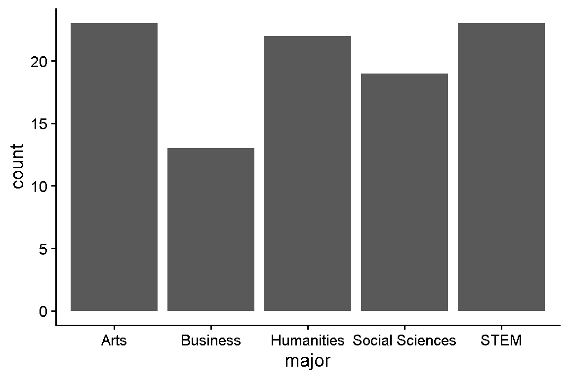
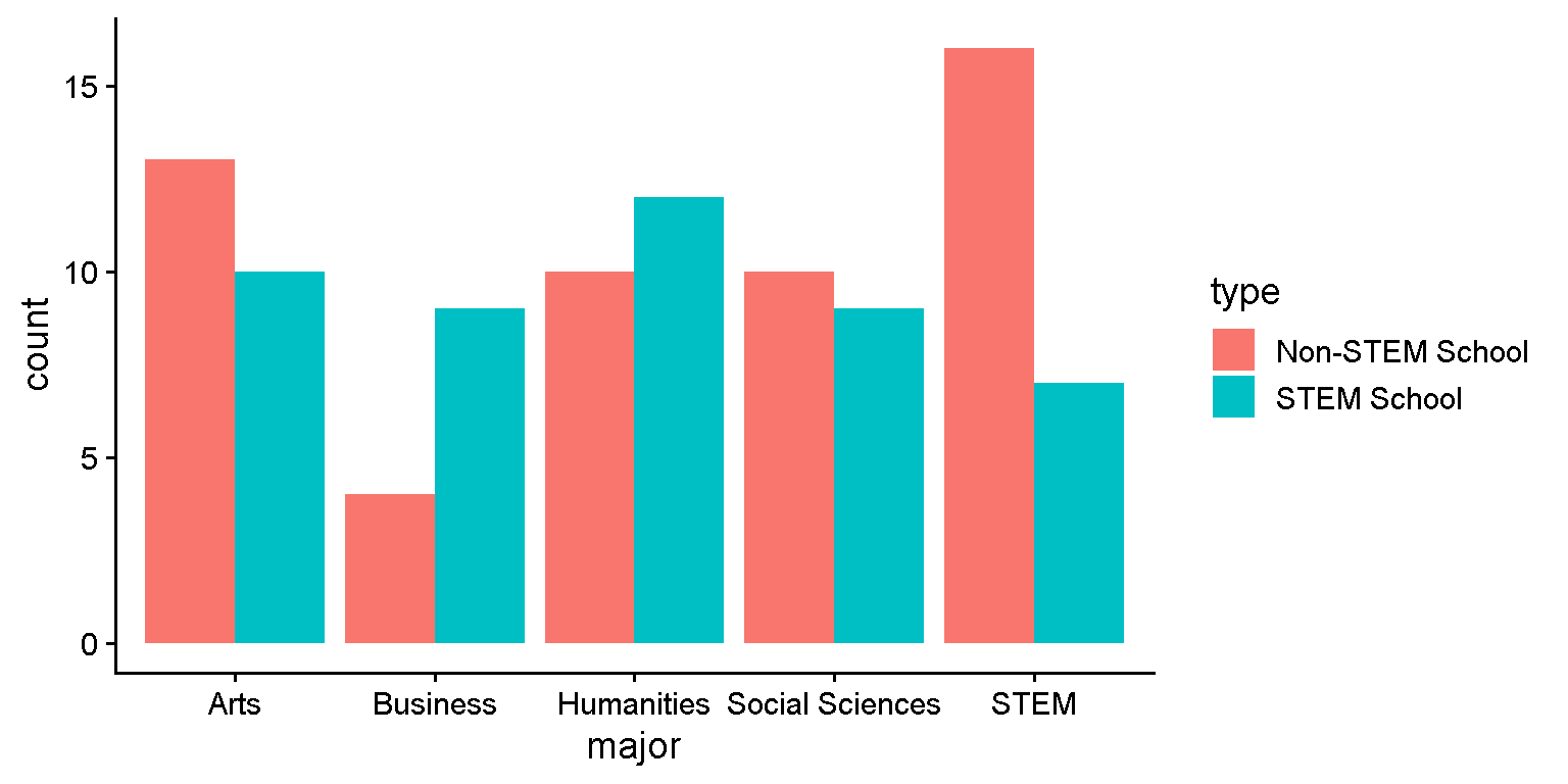
Working With Count Data: `geom_bar()`